In our previous post, we explored how to run a full machine learning experiment using PySyft to study heart disease. This time, we’ll take a step further by implementing a complete Federated Learning (FL) example, still working with the same medical datasets. The beast part? We’ll get it done with just 10 lines of code, using a new gem in the PySyft API. Plus, there is a bonus surprise in the end…Let’s dive in!
Federated Learning in a Nutshell
If you’re new to Federated Learning or need a refresher, here’s a quick overview:
Federated Learning (FL) enables collaborative model training across decentralized servers without sharing raw data. Instead of transferring data, each server sends model updates (e.g. gradients) to a central aggregator. The aggregator combines these updates to create an improved global model, whish is then shared back with each server. This process continues, with local models updating the global model without ever exchanging data. FL can be categorised into two main strategies based on how data is partitioned across servers: (1) Horizontal FL where servers have the same features but different samples, and (2) Vertical FL, where servers share data on the same samples but with different features. For this tutorial, we’ll focus on Horizontal FL, which is also the most common scenario.
FL with PySyft in 10 lines of Code
from collections import defaultdict

def avg(all_models_params: list[ModelParams]) -> ModelParams:
    return {param: np.average([p[param] for p in all_models_params], axis=0)
            for param in all_models_params[0].keys()}

fl_model_params, fl_metrics = None, defaultdict(list)  # one entry per epoch as a list
for epoch in range(FL_EPOCHS):
    for datasite in datasites:
        data_asset = datasite.datasets["Heart Disease Dataset"].assets["Heart Study Data"]
        metrics, params = datasite.code.ml_experiment(data=data_asset, model_params=fl_model_params).get()
        fl_metrics[epoch].append((metrics, params))
    fl_model_params = avg([params for _, params in fl_metrics[epoch]])
Each datasite runs a machine learning experiment (i.e. ml_experiment) using its own version of the “Heart Study Data” (lines 6-8). The experiment returns both performance metrics and local model parameters (line 8). After each epoch, all model parameters are averaged (line 10) using the avg function (line 3), which computes the aggregated model to be used in the next round of training.[1]
And the best part is: this approach is very flexible and works with any FL example using PySyft – you just need to adjust how you access the data_asset, and the specifics of the ml_experiment function.
💡 Note: The model parameters are stored as dictionaries of NumPy arrays, which is compatible with how model weights are saved in major deep learning frameworks like PyTorch. This makes the aggregation function generic and easy to integrate with other workflows.
Introducing the new MixedInputPolicy
You may have noticed that our ml_experiment function looks different from the other Syft functions you’ve seen. It not only takes input parameters linked to the assets on the datasite, but also accepts a dictionary of model parameters!
This is thanks to the new MixedInputPolicy introduced in the latest version of the PySyft APIs. This policy allows Syft functions to accept arbitrary parameters alongside datasite assets. Here is the definition of our ml_experiment function:
from syft import syft_function
from syft.service.policy.policy import MixedInputPolicy


@syft_function(
    input_policy=MixedInputPolicy(client=datasite, data=data_asset, model_params=dict)
)
def ml_experiment(data, model_params = None):
    """ML Experiment using a PassiveAggressive (linear) Classifier.
    Steps:
    1. Preprocessing (partitioning; missing values & scaling)
    2. Model setup (w/ `model_params`)
    3. Training: gather updated model parameters
    4. Evaluation: collect metrics on training and test partitions

    Parameters
    ----------
    data : pandas.core.DataFrame
        Input Heart Study data represented as Pandas DataFrame.
    model_params: ModelParams (dict[str, NDArrayFloat])
        ML Model Parameters as a dictionary of (paramenter_name, ndarray of float).

    Returns
    -------
    metrics : tuple[dict[str, float]]
        Evaluation metrics (i.e. MCC, Confusion matrix) on both training and test
        data partitions.
    model_params : ModelParams
        Update model params after training.
    """

    [...]
🔎 Note: If you’re curious about the finer details of setting up the ML experiment, here’s what you need to consider. First, we need to select a machine learning model that works with the averaging strategy we’re using to aggregate the model parameters. Linear models are ideal for this, so we’ll be using a
PassiveAggressiveClassifierfrom the Scikit-learn library. However, these models require clean, complete data, and as we discovered in the (Intro) Setup Datasites notebook, our dataset is quite sparse with missing values. To address this, we’ll need to preprocess the data to handle these gaps before training the classifier. The rate of missing data varies across the datasites, which may influence the overall training performance.
For the complete implementation of the ml_experiment function, and the full FL example to study heart disease, check out the new notebook added to the PySyft tutorial!
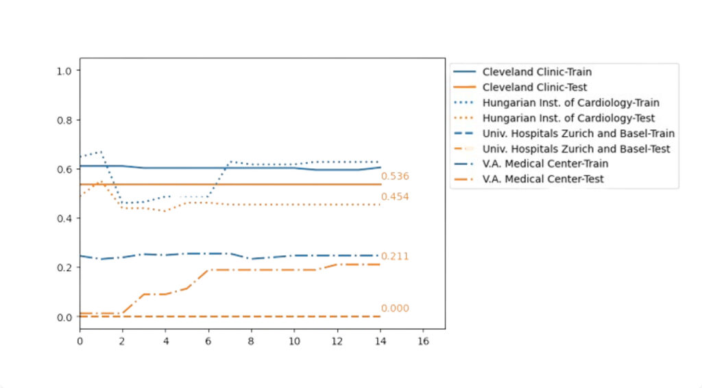
These are the results of the FL experiment to study heart disease using a (linear) PassiveAggressive Classifier:

Conclusions (and Bonus Highlights!)
As shown, we obtain a null MCC value for both training and testing on the data from “Univ. Hospitals Zurich and Basel,” which signals performance equivalent to random guessing. This outcome is likely due to the sparse nature of the data and the limitations of using a simple linear model, which struggles to capture the complexity of the problem.
A natural next step would be to explore how a more sophisticated, non-linear model like a Neural Network might perform on this dataset.
And what a better way to do this than by combining PySyft & PyTorch to run a new FL Experiment? You can find the complete Deep Learning Experiment example in the last notebook of the tutorial.
References
[1]The Human Use of Human Beings. Wikipedia. Retrieved [2024], from https://en.wikipedia.org/wiki/The_Human_Use_of_Human_Beings
